
When you create an index in PostgreSQL, you might think there’s just one type of index structure working behind the scenes. But PostgreSQL actually provides six different index types, each engineered for specific use cases with completely different internal structures and access patterns.
This is the final stop on our SQL Query Roadtrip. In the previous article , we explored how PostgreSQL’s execution engine uses the Volcano model to transform abstract query plans into concrete operations. Before that, we covered parsing, analysis, rewriting, and planning. Now we’re diving into one of the most critical components that makes all of this fast: indexes.
Understanding these index types isn’t just academic—it’s practical. Choosing the right index can transform a query from “timeout after 30 seconds” to “returns in 10 milliseconds.” Let’s explore what makes each one tick.
The Common Foundation: PostgreSQL’s Index Infrastructure
Before we dive into specific index types, let’s look at what they all share. PostgreSQL uses a clever design: all index types plug into the same framework, like different tools that fit the same universal handle. This pluggable architecture is called IndexAmRoutine (defined in src/include/access/amapi.h).
All PostgreSQL index types implement this same interface, which means they all need to provide functions for:
- Building the index
- Inserting new entries
- Searching for values
- Cleaning up during VACUUM
- Estimating query costs
But here’s what makes this interesting: while they share this interface, each index type has completely different internal structures. They don’t just vary in performance characteristics—they’re fundamentally different data structures solving different problems.
The Slotted Page Architecture
Now, here’s the foundation that makes all these indexes work: how PostgreSQL actually stores data on disk.
All indexes share PostgreSQL’s slotted page design for storage. Think of each 8KB page like a notebook page where you need to store items of different sizes. The challenge is: how do you organize them so you can find things quickly, use space efficiently, and handle deletions without leaving gaps everywhere?
PostgreSQL’s solution is clever. Instead of just writing data sequentially from start to end, it uses a two-sided approach:
At the front of the page, there’s a line pointer array—essentially a table of contents. Each pointer is small and fixed-size, saying “item #1 starts at byte 2047, item #2 starts at byte 1998” and so on. This array grows forward into the page as you add more items.
At the back of the page, the actual data (tuples) is stored, growing backward toward the front. Each tuple can be different sizes—some small, some large.
In the middle, you have free space. As you add items, the pointers grow forward and the data grows backward, eating into this free space. When they meet, the page is full.
Here’s what it looks like:
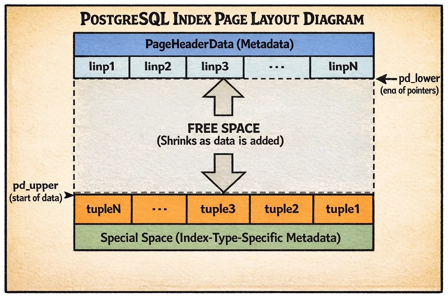
Let’s break down what you’re seeing:
- Top section: Page header (metadata) followed by the line pointer array growing downward
- Middle section: Free space that shrinks as you add more data
- Bottom section: The actual tuple data growing upward from the bottom
- Very bottom: Special space reserved for index-type-specific metadata
Why this design? Because pointers are fixed-size and small, you can binary search through them quickly to find a specific item. The actual data can be variable-sized and doesn’t need to move around when you delete items—you just update the pointer.
There’s also a special space at the very end where each index type stores its own custom metadata. For B-trees, this holds sibling page links. For hash indexes, it stores bucket information. This is where the different index types start to diverge in their implementation.
Now let’s explore each index type, starting with the workhorse of PostgreSQL indexing.
B-tree: The General-Purpose Champion
When you create an index without specifying a type, PostgreSQL creates a B-tree. It’s the default for good reason—it’s fast, versatile, and handles most use cases beautifully.
How It’s Structured
Think of a B-tree like a corporate hierarchy. At the top, you have executives (the root) who delegate to managers (internal pages), who delegate to individual workers (leaf pages) who do the actual work. When you’re looking for someone, you start at the top and follow the chain down.
The tree has multiple levels organized like this:
Leaf pages (level 0) are at the bottom. These store the actual index entries—each entry contains the indexed value (like a customer ID) and a pointer to where that row lives in the heap table. This is where the real data lives.
Internal pages are in the middle. They don’t store actual data—just signposts that say “values 1-100 are this way, values 101-200 are that way.” Each entry points down to a child page that handles a specific range of values.
Root page is at the top. It’s the starting point for all searches. It could be at any level—a small index might have the root directly pointing to leaf pages, while a huge index might have several layers of internal pages in between.
Here’s what makes PostgreSQL’s B-tree special: it uses the Lehman and Yao algorithm, which solves a tricky problem—how do you let multiple processes search and modify the tree simultaneously without everything grinding to a halt from locking?
The key innovation is adding horizontal links between sibling pages. Imagine if each manager in our corporate hierarchy also had a direct line to the manager next to them. This allows efficient range scans—once you find the first matching leaf page, you can just follow the sibling links sideways without going back up the tree. It also helps concurrent operations by reducing lock contention.
Here’s what a PostgreSQL B-tree looks like:
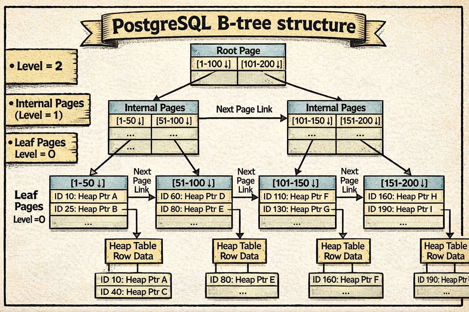
Notice how each level forms a horizontal chain through the sibling links (shown as the arrows connecting pages at the same level). The vertical arrows show parent-child relationships, while the horizontal links enable efficient range scans and concurrent access.
Each page stores some extra metadata in its special space to make this work (see BTPageOpaqueData structure). This metadata keeps track of:
- Sibling pointers (
btpo_prevandbtpo_next) that link each page to its neighbors on the left and right. These create horizontal chains at each level—all leaf pages are linked together in a chain, and all internal pages at each level form their own chains. - Tree level (
btpo_level) that indicates how far this page is from the leaves. Leaf pages are level 0, their parents are level 1, and so on. - Page flags that mark what type of page this is (root, internal, leaf, deleted, etc.)
- Cycle ID for detecting concurrent page splits—a clever trick that helps PostgreSQL know if the tree structure changed while a search was navigating down.
With this structure in place, let’s walk through how PostgreSQL actually navigates and modifies the tree.
How Access Works
For searches, B-tree descent is remarkably efficient. Starting from the root (which PostgreSQL keeps in memory almost all the time because it’s accessed so frequently), PostgreSQL:
- Reads the current page
- If the search key is greater than the page’s high key, follows the right-link (handling concurrent splits)
- Otherwise, binary searches within the page to find the appropriate child pointer
- Descends to that child and repeats
For a table with millions of rows, this typically means 3-4 page reads to reach a leaf, with the upper levels cached in memory. In practice, that’s often just 1-2 actual disk reads—the difference between 0.1ms (cached) and 10ms (from disk) for a query.
For range scans, once you find the first matching leaf entry, you just scan forward (or backward) through leaf pages using the sibling links. No tree re-descent needed.
For inserts, PostgreSQL descends to the appropriate leaf page and inserts the new tuple. If the page is full, it splits the page in two, creates a new high key, and inserts a downlink in the parent (which might recursively split all the way to the root).
Given B-tree’s versatility and efficiency, when should you reach for it versus the specialized index types?
When to Use It
B-tree is your default choice. Use it for:
- Equality queries (
WHERE id = 42) - Range queries (
WHERE created_at BETWEEN '2024-01-01' AND '2024-12-31') - Sorted results (
ORDER BY name) - Prefix matches (
WHERE name LIKE 'John%') - Unique constraints (B-tree is the only index supporting
UNIQUE)
B-tree’s complexity is O(log N) for searches, inserts, and deletes. For a billion-row table with good caching, you’re typically looking at 1-2 disk reads per lookup.
B-tree’s versatility makes it the default choice, but what if you only need equality lookups and want to skip the tree traversal entirely?
Hash: The Equality Specialist
If you only need equality comparisons and want slightly faster lookups, PostgreSQL offers Hash indexes. They implement a variant of linear hashing with overflow chaining—but what does that actually mean? Let’s break it down.
📜 Historical note: Hash indexes were long considered problematic in PostgreSQL (they weren’t WAL-logged until PostgreSQL 10, meaning crashes could corrupt them). They’re now fully reliable, but B-tree’s improvements over the years have narrowed the performance gap, making Hash indexes relevant only in very specific scenarios.
How It’s Structured
Imagine you’re organizing files into filing cabinets. Instead of keeping them in sorted order, you use a simple rule: take the file number, do some math on it, and that tells you which drawer to put it in. That’s essentially how hash indexes work.
Hash indexes use a hash table - a structure where you hash your value (like an ID) to get a bucket number, then look in that bucket. The beauty is that finding the right bucket is instant math, not searching.
But here’s the challenge: what happens when a bucket fills up? You can’t just resize the entire hash table—that would require rehashing everything at once, causing massive pauses.
PostgreSQL’s solution is linear hashing, which grows the table gradually. Instead of rehashing everything when the table gets too full, it splits just one bucket at a time. Here’s how it works:
- PostgreSQL tracks a “split point” bucket number
- When the overall load factor gets too high (default: 75%), it splits the bucket at the split point
- The split point advances to the next bucket
- This continues until all buckets in the current “level” have been split, then it starts over with a new level
This keeps things smooth and predictable—no huge pauses, just gradual growth.
But what actually happens during a split? Let’s walk through a concrete example. Say you have buckets 0-3 (using 2 bits to determine bucket: 00, 01, 10, 11), and you’re splitting bucket 0:
Before the split:
- Bucket 0 contains all values whose hash ends in binary
00(like hash values 4, 8, 12, 16…) - Buckets use 2 bits of the hash to determine placement
During the split:
- PostgreSQL creates a new bucket 4
- It re-examines every entry in bucket 0 using one MORE bit of the hash (3 bits instead of 2)
- Entries whose hash ends in binary
000stay in bucket 0 - Entries whose hash ends in binary
100move to the new bucket 4 - The split point advances to bucket 1 (which will be split next)
After the split:
- Bucket 0 now has half its original entries (those ending in
000) - Bucket 4 has the other half (those ending in
100) - When looking up a value, PostgreSQL checks: “Does this hash to a bucket number less than the split point?” If yes, use 3 bits. If no, use 2 bits.
This is the clever part: the hash table grows incrementally. Not all buckets use the same number of bits at the same time—buckets that have been split use one more bit than buckets that haven’t. When all buckets have been split, you have twice as many buckets, everyone uses the new bit count, and the cycle starts over at a new level.
Now let’s look at how PostgreSQL organizes the hash index on disk. Think of it like a physical filing system in an office with different types of storage:
Metapage (always block 0) is the control center. Open the hash index file, and the very first page tells you everything about the index configuration: how many buckets currently exist, what the maximum bucket number is, and where to find things. It’s like the directory at the entrance of a building—before you can navigate anywhere, you read this first.
Bucket pages are where the actual data lives. When you create a hash index, PostgreSQL allocates one primary page for each bucket. When you hash a value like customer ID 42 and it maps to bucket 7, that data goes into bucket 7’s primary page. These are your main storage locations.
Overflow pages are the expansion mechanism. Here’s the problem: what if bucket 7 gets popular and fills up completely? PostgreSQL creates an overflow page and chains it to the primary bucket page. Need more space? Add another overflow page to the chain. It’s like having expandable file folders—when the main folder gets full, you clip on an extension folder. All these pages link together so you can traverse the entire chain to find what you need.
Bitmap pages are the recycling system. When you delete data from the hash index, overflow pages might become empty. Rather than just forgetting about them, PostgreSQL tracks these free pages in bitmap pages—essentially a list saying “these overflow pages are available for reuse.” When bucket 7 needs a new overflow page, PostgreSQL checks the bitmap first before allocating a brand new page. This prevents the index from growing forever.
Here’s how all these pieces fit together:
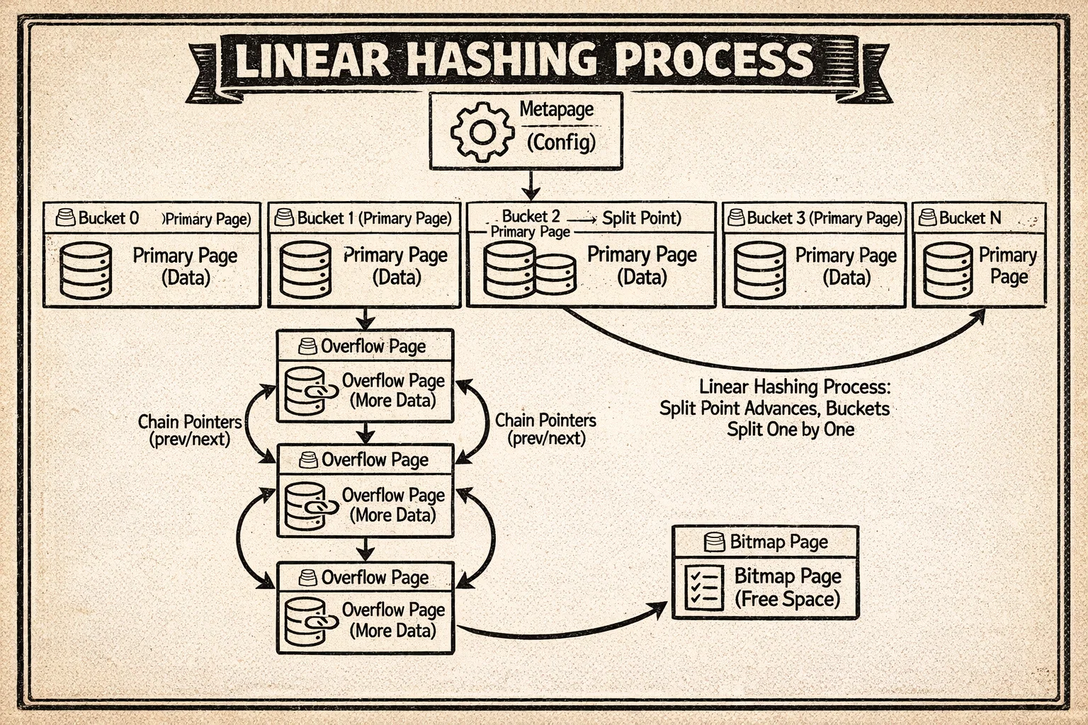
The diagram shows the metapage at the top, the bucket pages with their primary storage, overflow chains extending from busy buckets, and how the linear hashing split process redistributes data by adding new buckets and using one more bit of the hash value.
Each page stores metadata in its special space to maintain these chains (see HashPageOpaqueData structure). This metadata tracks:
- Chain pointers (
hasho_prevblknoandhasho_nextblkno) that link overflow pages together. If a bucket fills up and needs overflow pages, these pointers create a doubly-linked chain so you can traverse forward and backward through all pages belonging to that bucket. - Bucket number (
hasho_bucket) that identifies which bucket this page belongs to. This is essential when you’re traversing overflow chains—you need to know which bucket you’re working with. - Page flags that indicate what type of hash page this is (primary bucket page, overflow page, bitmap page, etc.)
The chain structure means if bucket 42 overflows, you can follow the links from its primary page through all its overflow pages in sequence.
Now let’s see how PostgreSQL uses this hash structure to handle inserts and lookups.
How Access Works
For inserts, PostgreSQL:
- Hashes your value using the type’s hash function (like
hashint4()for integers) - Maps the 32-bit hash to a bucket number using bit masking
- Finds the appropriate page in that bucket’s chain
- Binary searches within the page to maintain sorted order by hash value
- Inserts the tuple
If the table’s load factor exceeds the configured fill factor (default: 75), PostgreSQL triggers a bucket split: creates a new bucket, rehashes entries from one old bucket, and redistributes them.
For searches, it’s similar: hash the value, find the bucket, scan the bucket chain for matches. This is typically O(1) average case—just 1-2 page reads for a lookup.
So with all this complexity of linear hashing and bucket management, when does it actually make sense to use Hash over B-tree?
When to Use It
Hash indexes are surprisingly niche. The main advantage over B-tree is avoiding tree traversal—you go directly to the data. But the limitations are severe:
Hash is only useful for:
- Equality queries (
WHERE col = value) - Single-column indexes
- High-cardinality columns
Hash cannot handle:
- Range queries (
WHERE col > value) - Sorting (
ORDER BY) - Pattern matching (
LIKE) - Unique constraints
- Multi-column indexes
In practice, B-tree is often just as fast for equality queries (especially when upper tree levels are cached) and far more versatile. Hash indexes are a specialized tool—useful when you have a very specific equality-only workload and want to squeeze out every last bit of performance.
Hash handles simple equality well, but what about complex queries like “find all points within this region” or “which documents contain these words”? That’s where our next index type shines.
GiST: The Geometric Genius
GiST (Generalized Search Tree) isn’t a single index type—it’s a framework for building custom access methods. It’s particularly famous for powering PostGIS (spatial databases), but it handles much more.
How It’s Structured
Imagine you’re organizing a map collection. Instead of sorting maps alphabetically, you organize them by region: “Maps of Europe,” “Maps of Asia,” etc. But here’s the tricky part—some maps show regions that overlap (like “Mediterranean” which includes parts of Europe, Africa, and Asia). GiST is designed to handle exactly this kind of overlapping organization.
GiST implements an R-tree-like structure that’s similar to B-tree but with one critical difference: the ranges can overlap. This is essential for spatial data like geographic coordinates, where bounding boxes naturally overlap.
The tree structure looks familiar:
Leaf pages store the actual index entries—things like “this polygon” or “this point”—along with pointers to where those rows live in the heap table.
Internal pages don’t store actual data. Instead, they store bounding predicates—descriptions of what’s below them. For geometric data, this might be a bounding box: “everything in this subtree is somewhere inside this rectangle.” For range types, it might be “all ranges in this subtree overlap with this interval.”
Root page is always at block 0, the starting point for searches.
The key insight: unlike B-tree where you know exactly which child to follow (values 1-100 go left, 101-200 go right), with GiST you might need to check multiple children because their bounding predicates can overlap. Searching for “points near the Mediterranean” might mean following paths into both the Europe and Africa subtrees.
Here’s what a GiST tree looks like:
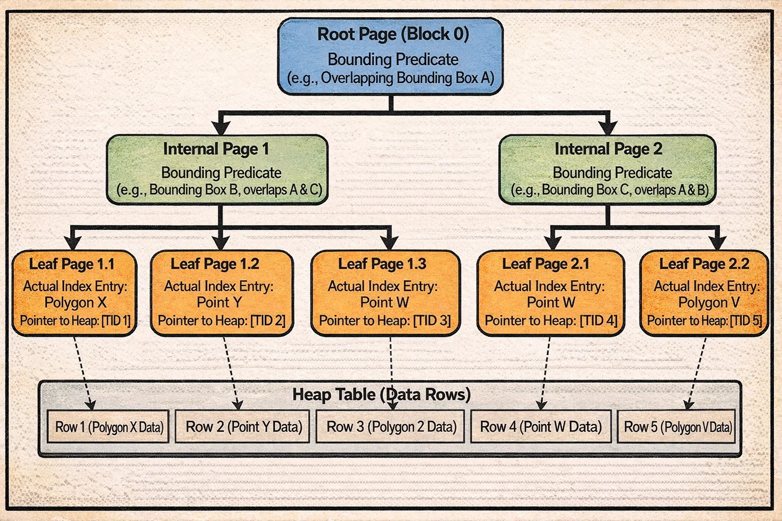
Notice how the bounding boxes at the internal level can overlap—this is the key difference from B-tree. A search might need to descend into multiple subtrees because the query region intersects with multiple bounding boxes. The right links between sibling pages (like B-tree) help with concurrent access.
Each page stores some metadata (see GISTPageOpaqueData structure) to handle concurrent access and navigation:
- Node Sequence Number (NSN) is a special kind of timestamp that gets updated only when a page splits. When PostgreSQL is descending the tree, it can compare the parent’s LSN (log sequence number) with the child’s NSN. If the parent’s LSN is less than the child’s NSN, that means the child split while the search was in progress—so PostgreSQL knows it needs to follow the rightlink to find all the data.
- Right link points to the next sibling page, creating horizontal chains just like B-tree. This helps with concurrent operations and range scans.
- Page flags indicate whether this is a leaf page, internal page, or has been deleted.
The NSN is particularly clever—it solves the problem of detecting concurrent page splits without requiring expensive locking during searches.
Now that you understand GiST’s tree structure, let’s see how PostgreSQL actually uses it for queries and inserts.
How Access Works
GiST is extensible—different data types need different logic for organizing data. To make this work, each GiST operator class provides support functions that tell PostgreSQL how to handle that specific type of data. Let’s look at the key ones:
Consistent: “Does this bounding predicate match my search query?” For geometric data, this might check if a bounding box overlaps with the search area.
Union: “If I combine these predicates, what’s the smallest bounding predicate that contains all of them?” For geometric data, this creates the smallest rectangle that contains all the child rectangles.
Penalty: “If I add this new entry to this subtree, how much do I need to expand its bounding predicate?” For geometric data, this calculates how much bigger the bounding box would need to become.
PickSplit: “When this page is full and needs to split, how should I divide these entries into two groups?” The goal is to minimize overlap between the two resulting groups.
Now let’s see these functions in action.
For searches, imagine you’re looking for “all restaurants within this neighborhood” (represented as a search box):
- Start at the root and check each child’s bounding box using Consistent
- If a bounding box overlaps your search area, descend into that child
- Here’s the key difference from B-tree: you might need to follow multiple children because their bounding boxes can overlap your search area
- At the leaf level, check each actual point/polygon against your query
- Return all matches
If your search box touches three different bounding boxes at the root level, you’ll follow three paths down the tree. With lots of overlap, this can become expensive.
For inserts, let’s say you’re adding a new restaurant location:
- Start at the root and evaluate each child subtree using Penalty
- “If I add this point to this subtree, how much bigger does its bounding box need to become?”
- Choose the child with the smallest penalty (minimal expansion needed)
- Descend into that child and repeat until you reach a leaf
- Insert the new entry into the leaf page
- If the page is full, use PickSplit to divide the entries into two groups that minimize overlap
- The split might propagate up the tree (just like B-tree)
The quality of your PickSplit function makes all the difference. A good split creates clean, non-overlapping groups. A bad split creates lots of overlap, which means searches have to follow more paths and performance degrades.
Understanding GiST’s overlapping predicate structure reveals which problems it solves best.
When to Use It
GiST shines for:
- Geometric queries: Points, polygons, circles (via PostGIS)
- Range types: Checking if ranges overlap or contain values
- Network addresses: inet/cidr indexing
- Nearest-neighbor queries:
ORDER BY distance
The performance is O(log N) when predicates are well-separated, but can degrade toward O(N) if there’s high overlap. The quality of your operator class’s Penalty and PickSplit functions makes all the difference.
GiST excels at overlapping predicates for spatial data, but what about the opposite scenario—when you need to find rows containing any of many possible values, like words in a document or elements in an array?
GIN: The Inverted Index Master
GIN (Generalized Inverted Index) flips the normal index model on its head. Instead of mapping rows to their values, it maps values to rows. This makes it perfect for composite values where each row contains multiple keys.
How It’s Structured
Think about how you’d index a book. In a normal index, you look up a page number to find content. But what if you want to search by any word in the book? You’d need an inverted index—a list where each word points to all the pages it appears on. That’s exactly what GIN does.
GIN uses a two-level structure:
Entry Tree (B-tree of keys)
    ↓
Posting Lists/Trees (row locations for each key)
Here’s how it works:
The entry tree is a B-tree that stores all the unique keys that have been extracted from your data. For full-text search, these are words. For an array column, these are the individual array elements. For JSONB, these might be keys or values from the JSON documents.
Each entry in this tree points to a list of row locations (TIDs - tuple IDs) where that key appears. But here’s where it gets clever: depending on how common the key is, PostgreSQL uses different storage:
Posting list: For keys that appear in just a few rows (the current threshold is around 384 bytes of TID data, roughly 64 rows), PostgreSQL stores a simple compressed array of TIDs. It’s compact and fast to scan.
Posting tree: For keys that appear in many rows (like the word “the” in a full-text index, which might appear in millions of documents), a simple list would be huge and slow to search. So PostgreSQL builds a separate B-tree just for that key’s TIDs. Now searching within those locations is efficient even if there are millions.
PostgreSQL automatically converts posting lists to posting trees when they grow beyond the threshold. You don’t have to think about it—it adapts to your data.
There’s also a pending list—a separate structure where new index entries accumulate in fast update mode before being merged into the main index. This makes bulk inserts much faster (we’ll explore exactly how in the next section).
Each GIN page stores minimal metadata (see GinPageOpaqueData structure)—intentionally kept small at just 8 bytes:
- Right link points to the next page, allowing pages to be chained together
- Max offset tracks the number of items on the page (meaning varies by page type)
- Page flags indicate what type of GIN page this is: entry tree page, posting tree page, pending list page, or metapage
The small metadata footprint is deliberate—GIN pages need to pack in as much actual data as possible since they’re storing potentially millions of posting entries.
Here’s how the GIN structure looks:
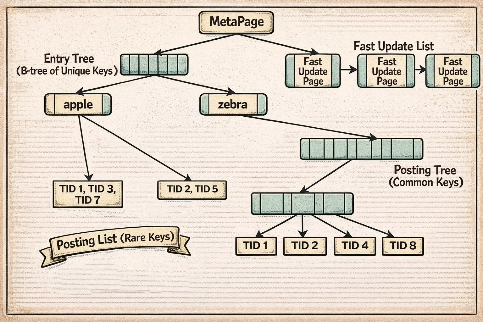
The diagram shows the entry tree (a B-tree of unique keys) at the top, with each entry pointing to either a posting list (for infrequent keys) or a posting tree (for common keys). The pending list on the side accumulates new entries in fast update mode before being merged into the main structure.
Understanding this two-level structure helps explain why GIN has different performance characteristics for inserts versus searches.
How Access Works
For inserts, GIN has two modes:
Fast update mode (default): New entries go into a pending list—an unsorted list of entries waiting to be merged. When the pending list fills up (default: 4MB), it’s sorted and merged into the main index in one batch. This makes bulk inserts 10-100x faster by reducing the number of tree modifications.
The trade-off: searches have to scan this unsorted pending list in addition to searching the main index. For a 4MB pending list with hundreds of thousands of entries, this might add 10-50ms to query time. Once the pending list is merged (which happens automatically), queries are fast again.
Direct insert mode: Each key is immediately inserted into the entry tree and its posting list/tree. Slower for inserts (because every insert modifies the main tree structure), but searches don’t pay the penalty of scanning the pending list.
For searches:
- Extract keys from your query (e.g., for “postgres & search”, extract [‘postgres’, ‘search’])
- Look up each key in the entry tree (O(log N))
- Retrieve the posting list/tree for each key (O(log P) + O(P) where P = matches)
- Combine the TID lists according to your query logic (AND, OR, NOT)
- Scan the pending list (if using fast update mode)
This inverted index structure makes GIN the natural choice for certain types of queries.
When to Use It
GIN is the go-to index for:
- Full-text search: tsvector columns
- Array operations:
@>,&&,<@operators - JSONB queries: Key existence, path lookups, containment
- Any multi-key data: Each row contains multiple values to index
The space efficiency is remarkable. For full-text indexing, GIN is typically 10-50x smaller than creating B-tree indexes on all possible terms.
GIN’s strength is handling composite values with its inverted index, but what if you have data that naturally partitions into non-overlapping regions, like IP addresses or text prefixes?
SP-GiST: The Space Partitioner
SP-GiST (Space-Partitioned GiST) is designed for non-overlapping partition structures like tries, quad-trees, and k-d trees. Unlike GiST where predicates can overlap, SP-GiST ensures each search follows exactly one path through the tree.
How It’s Structured
SP-GiST is actually a framework that can implement different tree structures depending on what you’re indexing. It’s like having a customizable filing system where you pick the organization scheme that fits your data best.
The key principle: at each level of the tree, data is partitioned into non-overlapping groups. Unlike GiST where ranges can overlap (requiring multiple paths), SP-GiST ensures there’s always exactly one path to follow when searching.
Here are the main structures it can implement:
For text data (tries/radix trees):
Imagine organizing words by breaking them down character by character. The root splits by first letter (a-z), then by second letter, and so on.
- Inner tuples store the common prefix shared by everything below them, plus pointers to children labeled by the next character. For example, a node might store “comp” with children for “computer” (going to ‘u’) and “complete” (going to ’l’).
- Leaf tuples store the remaining suffix of the actual string.
For 2D points (quad-trees):
Think of dividing a map into four quadrants (northwest, northeast, southwest, southeast), then dividing each quadrant into four more, and so on.
- Inner tuples store a centroid (center point) and have exactly 4 children, one for each quadrant.
- Leaf tuples store the actual points.
For 2D points (k-d trees):
Imagine splitting space alternately by X and Y coordinates. Level 1 splits by X, level 2 by Y, level 3 by X again, and so on.
- Inner tuples store a splitting coordinate value and have 2 children (left/right or above/below depending on the level).
- Leaf tuples store the actual points.
The beauty of SP-GiST is that it’s extensible—you can implement custom partition schemes for your own data types while reusing the core framework.
Here’s what an SP-GiST tree looks like:
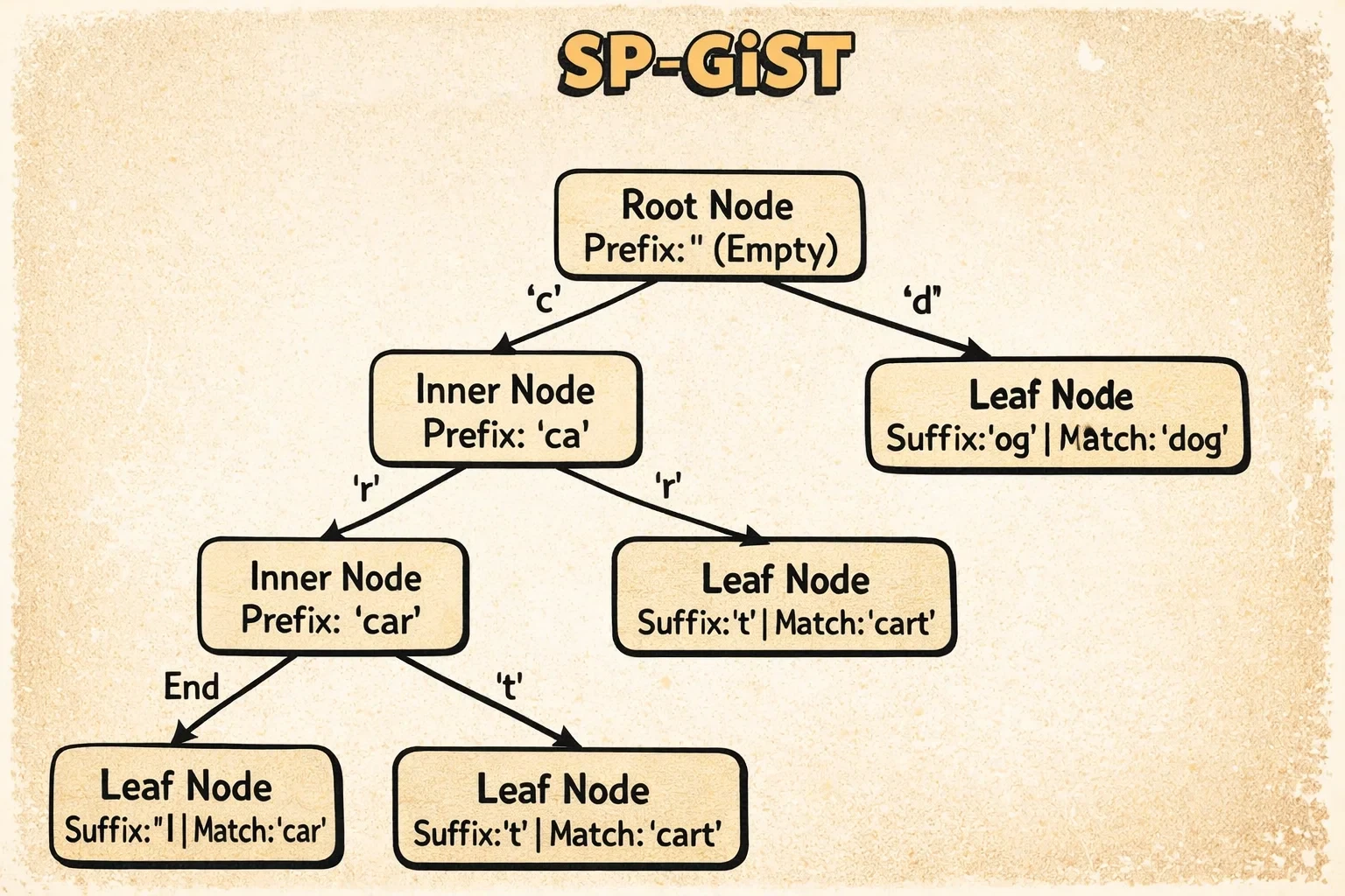
The diagram shows how SP-GiST implements a radix tree for text. Inner tuples contain a prefix (like “comp”) and labeled pointers to children (like ‘u’ for “computer” or ’l’ for “complete”). Each search follows exactly one path through the tree based on the prefix and labels—no overlapping regions, no backtracking.
Each SP-GiST page stores metadata (see SpGistPageOpaqueData structure) that’s unique to its needs:
- Page flags indicate what type of page this is (inner node page, leaf page, null-storing page, or metapage)
- Redirection count tracks the number of redirection tuples on this page—these are special pointers used when inner nodes need to move during page splits
- Placeholder count counts placeholder tuples, which are temporary markers left during incomplete operations that need to be cleaned up later
- Page ID is always
0xFF82, a magic number that helps tools identify this as an SP-GiST page
The redirection and placeholder tuples are SP-GiST’s way of handling the complexity of splitting pages in non-overlapping partition trees—it’s trickier than B-tree splits because you can’t just split anywhere, you need to maintain the partition structure.
The real magic of SP-GiST becomes clear when you see how searches navigate through these non-overlapping partitions.
How Access Works
The key insight is single-path descent. When searching, the operator class’s functions determine exactly which child to follow at each level. No backtracking, no multiple paths.
For text prefix searches using tries:
- Match prefix characters from root to leaf
- Follow exactly one child per level based on character value
- Complexity is O(k) where k = string length (independent of table size!)
For point searches using k-d trees:
- At each level, compare against the splitting coordinate
- Go left or right (alternating x/y dimensions by level)
- Complexity is O(log N) for balanced trees
This single-path descent property makes SP-GiST ideal for specific types of data and queries.
When to Use It
SP-GiST is perfect for:
- Text prefix searches:
WHERE name ^@ 'John'(starts with) - IP address hierarchies: inet/cidr ranges
- 2D point queries: Using k-d trees (often faster than GiST)
- Any non-overlapping partition scheme
The radix tree for text is particularly elegant—search time depends only on string length, not table size.
All the indexes we’ve seen so far index individual rows or values. But what if your table is massive and your data has natural ordering? That’s where our final index type takes a radically different approach.
BRIN: The Block Range Index
BRIN (Block Range Index) is radically different from every other index type. Instead of indexing individual tuples, it stores summary information about consecutive ranges of heap blocks.
⚠️ Critical requirement: BRIN only works well if your data has physical correlation—meaning the order values are stored on disk matches their logical order. If you have log entries inserted chronologically, timestamp values will be physically ordered (high correlation). If you have randomly inserted customer IDs, they’ll be scattered across the table (low correlation). We’ll come back to this with examples in a moment.
How It’s Structured
BRIN takes a radically different approach from other indexes. Instead of indexing individual rows, it indexes ranges of pages and stores summary information about each range.
Imagine you have a diary that spans 10 years. Instead of indexing every single entry, you could write on the spine of each notebook: “January 2020 - March 2020.” When you’re looking for something from February 2020, you know exactly which notebook to grab. That’s BRIN.
Here’s how it works:
BRIN divides your table into consecutive chunks of pages (default: 128 pages per chunk). For each chunk, it stores a summary:
Heap blocks:  [0-127] [128-255] [256-383] ...
BRIN ranges:     R0        R1        R2    ...
Summaries:   [min,max] [min,max] [min,max] ...
For numeric data (minmax operator class), each summary just stores the minimum and maximum values found in those 128 pages. So if pages 0-127 contain customer IDs ranging from 1 to 5000, the summary stores [1, 5000].
For range types (inclusion operator class), it stores the union of all ranges in that chunk.
When you search for a value, PostgreSQL scans through these summaries (not the actual data) and says “this range might contain my value, this one definitely doesn’t, this one might…” Then it only reads the “might contain” page ranges and checks each row.
The reverse map (revmap) is a lookup table that lets PostgreSQL quickly find which summary tuple describes a given page. It’s O(1)—just direct access.
The trick: this only works well if your data is physically ordered. If customer IDs 1-5000 are scattered randomly across the table, every range will have summary [1, 5000] and BRIN provides no filtering. But if you insert data in order (like timestamps), the ranges have tight, non-overlapping summaries.
Unlike other index types, BRIN doesn’t use standard page opaque data. Instead, it has a unique page organization (see BrinMetaPageData structure):
- Block 0 is a metapage that stores configuration like how many pages are in each range (
pages_per_range) and where the last reverse map page is. It also has a magic number (0xA8109CFA) for identification. - Subsequent blocks are revmap pages (reverse map) that provide O(1) lookup from any heap block number to its summary tuple. This is what makes BRIN inserts and lookups so fast—no tree traversal needed.
- Remaining blocks store summary tuples, which are the actual min/max (or other summary) values for each range.
This structure is radically simpler than B-tree or GiST—there’s no tree, no sibling links, no complex navigation. Just direct access through the revmap.
Here’s how BRIN organizes data:
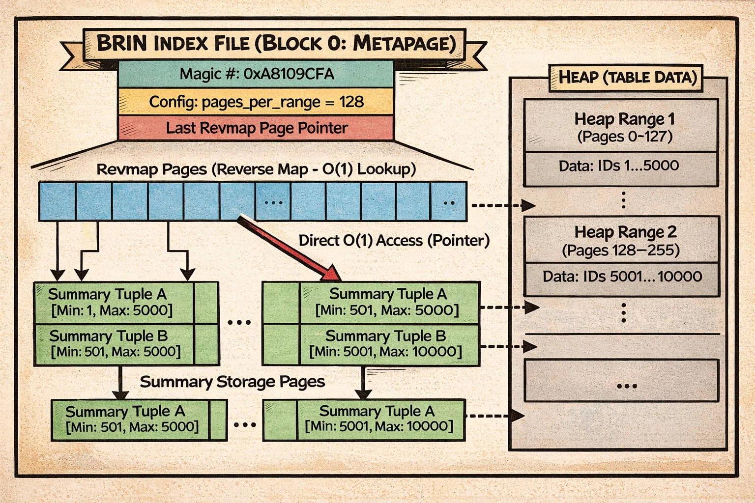
The diagram shows the metapage at block 0, followed by revmap pages that provide O(1) lookup from heap block ranges to their summary tuples. The summaries store min/max values (or bloom filters, or range unions) for consecutive chunks of heap pages. Notice how the entire structure is flat—no tree traversal, just direct lookup through the revmap.
This simple flat structure makes BRIN’s operations remarkably straightforward compared to tree-based indexes.
How Access Works
For inserts, BRIN is remarkably fast: O(1). It just updates the min/max for the affected range. No tree rebalancing, no complex data structures.
For searches, BRIN scans all range summaries sequentially:
- Read the revmap
- For each range, check if the summary is consistent with the query
- If yes, add the entire 128-page range to a bitmap
- Return a lossy bitmap (page ranges, not individual TIDs)
The bitmap heap scan then reads those page ranges and rechecks each tuple.
The Correlation Requirement
Here’s the critical insight: BRIN only works well if your data is physically ordered. If values correlate with their physical location (correlation > 0.5), BRIN can exclude most ranges. If data is randomly distributed (correlation near 0), BRIN provides almost no filtering—you’ll scan the entire table.
Perfect use case: time-series data. If you insert log entries chronologically and query by timestamp, BRIN’s summaries will be tight. A query for “last week’s data” might only match 1-2 ranges out of thousands.
With this correlation requirement in mind, here are the scenarios where BRIN excels.
When to Use It
BRIN is ideal for:
- Very large tables (>10GB) with natural ordering
- Time-series data: Timestamps, log tables, IoT sensors
- Append-only workloads: Data inserted in order
- Range queries on correlated columns
The space efficiency is stunning—a BRIN index can be 10,000x smaller than B-tree. For a 1TB table, BRIN might be 4MB while B-tree would be 100+GB.
But remember: check correlation first using pg_stats.correlation. If it’s below 0.5, B-tree is likely better.
The Index Comparison Matrix
Let’s put it all together. Here’s how these indexes stack up:
Notation guide:
N= number of rows in the tableK= number of matching rowsP= number of predicates to check (for GiST, can be > 1 due to overlap)R= number of block ranges in the indexk= length of the search key (for SP-GiST trie)
| Index Type | Best For | Structure | Typical Size | Equality | Range | Ordering |
|---|---|---|---|---|---|---|
| B-tree | General purpose | Balanced tree | 10-20% of table | O(log N) | O(log N + K) | Yes |
| Hash | Exact equality | Hash buckets | 10-15% of table | O(1) | No | No |
| GiST | Spatial, full-text | R-tree variant | 15-30% of table | O(log N × P) | Yes | Distance |
| GIN | Arrays, JSONB, text | Inverted index | 5-50% of table | O(log N + K) | No | No |
| SP-GiST | Tries, partitions | Space partition | 10-25% of table | O(k) or O(log N) | Limited | Distance |
| BRIN | Time-series | Block summaries | 0.001% of table | O(R) | O(R) | No |
Wrapping Up
PostgreSQL’s six index types aren’t just performance variations—they’re fundamentally different data structures solving different problems. B-tree’s balanced tree handles general queries. Hash’s bucket structure optimizes equality. GiST’s overlapping predicates enable spatial queries. GIN’s inverted index makes full-text search possible. SP-GiST’s partitioning provides single-path descent. BRIN’s summaries compress gigabytes into megabytes.
Now that you understand how each index type works internally—their structures, access patterns, and trade-offs—you’re equipped to explore them in your own applications. The best way to internalize this knowledge is to experiment: create different index types on your data, run EXPLAIN ANALYZE on your queries, and measure the performance differences. What works best depends entirely on your specific data characteristics and query patterns. A GIN index might be perfect for one use case while a B-tree serves another better, and there’s no substitute for hands-on evaluation with your actual workload.
Understanding these structures also helps you recognize when something’s wrong. If a query with a “perfect” index is still slow, you can now reason about why—maybe GiST predicates are overlapping heavily, or BRIN’s correlation assumption doesn’t hold for your data, or GIN’s pending list has grown too large. You’re no longer just following best practices blindly; you understand the mechanisms behind them.
And that concludes our SQL Query Roadtrip! We’ve journeyed through parsing, analysis, rewriting, planning, execution, and now indexes. You’ve seen how PostgreSQL transforms your SQL text into optimized execution plans and produces results. The next time you run a query, you’ll understand the entire journey—from the moment you hit Enter to the instant results appear on your screen.
The internals are fascinating, but remember: this knowledge serves a purpose. It helps you write better queries, design better schemas, and debug performance issues with confidence. PostgreSQL is doing remarkable work behind the scenes, and now you know how it all fits together.